A Case-Based Complexity Approach to Health Inequality:
Understanding and Tracing Place-Based Differences to
enhance policy calibration
COMPLETE DATASET USED FOR STUDY
For details on the methods and rationale for dataset, see the article and below.
· Here is the link to the Complete Data: https://art-sciencefactory.com/COMPLEXIT_CompleteData.xlsx
o It contains the SOM node (1 through 25) and SOM cluster solution (1 through 5) for each of the N=141 LAs,
along with their profile across all N=40 explanatory variables.
· Here is the link to COMPLEX-IT https://www.complex-it-data.org/
· See ANALYSES (below) for a more detailed understanding of what a SOM NODE ID and SOM CLUSTER ID mean in the
dataset and about how to interpret your results in COMPLEX-IT.
· Here are links to further information on the N=40 factors we examined in our study
· Dataset
– Links to help learn more about the HLE trend data and the N=40 factors in the
dataset
o
School
Readiness percentage of Free School Meals
o
First
time entrants to the youth justice system
o
First
time offenders per 100,000
o
Violent
offences per 1,000 population
o
16–17-year-olds
not in education, employment or training (NEET)
o
Employment
Gap Rate for those with long-term health condition
o
Percentage
of people in employment
o
Adults
in mental health services with stable living conditions
o
Domestic
abuse-related incidents and crimes
o
Sexual
offences per 1,000 population
o
Fuel
poverty (low income, high-cost methodology)
o
Social
Isolation: percentage of adult social care users
o
Under
18s conception rate / 1,000
o Indices
of Multiple Deprivation (IMD) - Average score
o
Indices of Multiple Deprivation (IMD) -
Proportion of LSOAs in most deprived 10% nationally
o
Percentage
of cancers diagnosed at stages 1 and 2
o
Cumulative
percentage aged 40-74 who received an NHS Health check
o
Mortality
from preventable causes
o
Mortality
cardiovascular preventable
o
Mortality
cancer preventable
Notes for those wanting to explore the
dataset or use for other studies
· Running a SOM solution in COMPLEX-IT will produce different results, as the software uses random initialization
and cluster solutions do vary slightly from one run to the next. As a result, repeated runs can yield slightly different maps.
However, with the same settings the overall topology fit (quantization/topographic error) should remain reasonably similar.
· Also note that when applying hierarchical clustering to the SOM’s prototypes, the numeric cluster labels are arbitrary, as
a different seed may rename clusters and re-label some cases, but the underlying groupings should effectively be the same.
· For a detailed overview of the SOM package, developed by Nathalie Vialaneix and her team, and as used in COMPLEX-IT,
see https://sombrero.clementine.wf/articles/c-doc-numericSOM.html
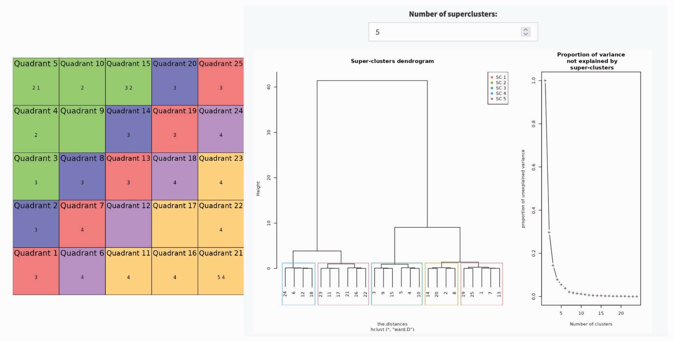
Figure 1: COMPLEX-IT results – SOM grid, dendrogram, and proportion of
variance
Steps in a Case-Based Complexity (CBC) used for the current study
(Note: these steps are
not the only one in COMPLEX-IT or CBC as there are a variety of tools
– for more, see Castellani
and Gerrits 2024, The Atlas of Social Complexity)
Analyses
Our analytic strategy followed a case-based
complexity (CBC) approach, operationalised through COMPLEX-IT,
an R-Shiney, online,
computational modelling, interdisciplinary methods platform (Schimpf
& Castellani 2020).
For our study we
employed a combination of machine learning, known as the self-organising map
(SOM) neural net,
and a SOM hierarchical
clustering technique. In previous studies we have conducted, this approach has
proven
better than other approaches, including time-series hierarchical regression, growth mixture modelling,
and latent class growth analysis
(Castellani
et al 2016; Castellani et
al, 2018).
Objective: The goal was to (a) cluster the major and minor trends in our healthy life expectancy trajectories
(HLE, 2011–2023) for our N=141 English local authority administrative areas (LAs); (b) identify which configuration
of N=40 factors (organised into social determinants, deprivation indices, preventable health outcomes) helped to
account for these different trends; and (c) examine these configurations in detail to develop a narrative for each
cluster trend — that is, a clear account of how different combinations of factors were associated with each cluster trend
and what these patterns suggest for policy and practice.
Step 1: To generate the hierarchical clusters, the SOM first requires a trained self-organising map. The strength of the SOM
is that it easily handles complex nonlinear mappings of complex trend data, making it an advance on more simplistic
trend fitting approaches, such as
k-means, growth mixture modelling, latent class growth analysis, and generalized
additive models (Castellani et al 2014; Jain 2010). In practice, this means we begin by running the SOM to organise
the HLE trajectories for all N=141 LAs across its grid. As shown on the left-hand side of Figure 1, we went with a
conventional 5×5 SOM grid, which treats the HLE data, initially, as comprised of 25 clusters called nodes, each representing
a unique HLE trend. The SOM places the N=141 LAs variously across these 25 nodes according to similar HLE profiles.
The result is that across the 25 nodes (clusters) of the 5X5 SOM grid, all N=141 LAs are located, providing the most
granular cluster map of the data, N=25
clusters.
Step 2: After the SOM arranges the N=141 LAs on the grid across all 25 clusters (nodes), its hierarchical clustering
technique helps us step back: it gathers similar nodes (clusters) into higher-level clusters, turning the detailed map into
a set of clear, interpretable HLE cluster trends. The strength of SOM hierarchical clustering is that, unlike k-means, it
does not impose a fixed number of clusters. Instead, it reveals how the 25 nodes cluster at successive levels of complexity.
For us, this meant identifying the major clusters as well as the smaller but still policy-relevant clusters in our dataset
– as clustering techniques do not, by convention, seek even distribution of cases across clusters (Jain 2010).
Once the cluster solution is settled on, three measures are used to determine the overall level of fit. Quantization error
measures how well the map represents the data: it is the average distance between each case and the node it is
mapped to. Topographical error measures how well the SOM preserves the data’s neighbourhood structure
– specifically, the proportion of cases whose
first and second best-matching units are not adjacent on the grid.
Lower values for both validity tests indicate a better-fitting map. In addition, the standard deviations of the cases around
each cluster are inspected to evaluate their respective homogeneity of variance. This is important for determining
how well the subsequent interpretation of the HLE trends can be trusted – higher levels of homogeneity support
more valid and reliable conclusions.
Step 3: With the cluster trends catalogued, we next sought to examine what configuration (i.e., profile) of
N=40 factors (i.e., social determinants, deprivation indices, preventable health outcomes) were associated with each
of the major and minor HLE clusters we identified in Step 2. For each HLE cluster trend we took the average (mean)
for each of our N=40 factors for all LAs (cases) associated with each cluster, resulting in the profiles shown in Table 1.
Step 4: Finally, we used these profiles to name the clusters and interpret each trend, tracing how the underlying
combination of factors helps make sense of the trajectory and its policy implications. We used standard qualitative
interpretive techniques to name and explore the clusters, treating each profile as a configuration of social
determinants, preventable health outcomes, and deprivation indices, and then synthesising these patterns into labels
and narratives that speak directly
to policy and practice.